Understanding Stationarity in Time Series

If you’ve ever tried to predict the weather, forecast stock prices, or model something like COVID-19 cases, you’ve likely encountered time series analysis. Time series is the statistical method used to forecast future values based on past data. But before we dive into the world of predictions, there’s a crucial concept to grasp: stationarity.

What is Stationarity?

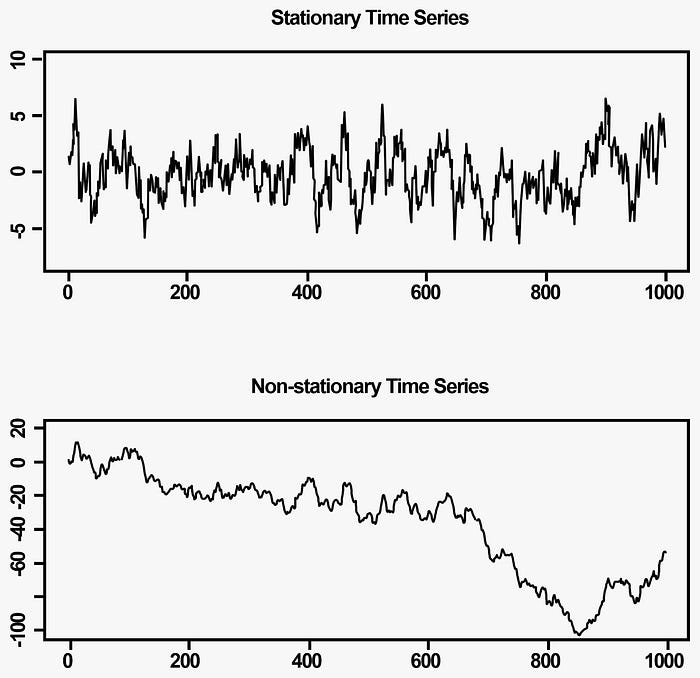
Imagine trying to build a forecasting model with data that behaves unpredictably—shifting averages, rising trends, or sudden spikes. It’s nearly impossible to predict the future with this kind of data. This is where stationarity comes in.

In simple terms, a stationary time series has consistent statistical properties over time. This means its mean, variance, and autocovariance remain constant. Mathematically, for a time series ( $\Delta X_t$ ), the mean and variance must be independent of time:

E[X_t] = \mu, \quad \text{Var}(X_t) = \sigma^2 \quad \text{for all } t

Think of it like a solid foundation for your predictive model. Without stationarity, your forecasts could easily be off-track.

Why Does Stationarity Matter?

Most time series models, including AR (Autoregressive), MA (Moving Average), and ARMA (a combination of both), rely on the assumption that your data is stationary. Without this assumption, the models may produce unreliable predictions.

Luckily, if your data is non-stationary, there are ways to fix it. One common method is differencing. This involves subtracting the previous value from the current one, which helps eliminate trends and make the data more stable.

Differencing Formula

The first difference of a time series ( $\Delta X_t$ ) is given by:

\Delta X_t = X_t - X_{t-1}

If the data still exhibits trends after differencing once, a second difference can be applied:

\Delta^2 X_t = \Delta X_t - \Delta X_{t-1}

This process can continue for higher-order differencing if needed.

Identifying Trends & Seasonality

You’ve probably seen time series data where the values steadily increase or decrease, or perhaps the data follows a repeating cycle over time. This is known as trends or seasonality, and it violates the stationarity rule.

To work with non-stationary data, we often need to detrend it, which means removing the underlying trend or seasonality. By doing this, we can focus on the more predictable, stationary parts of the data that are useful for forecasting.

Choosing the Right Model

Once you’ve made sure your data is stationary, it’s time to choose the appropriate forecasting model. Here’s a quick rundown of the most common models:

AR (Autoregressive): Uses past values (lags) to predict future values.
MA (Moving Average): Uses past errors (forecast mistakes) to make predictions.
ARMA (Autoregressive Moving Average): A combination of both AR and MA.

To determine which model is the best fit for your data, we can use diagnostic tools like ACF (Autocorrelation Function) and PACF (Partial Autocorrelation Function) plots. These plots reveal patterns in the data, which help us select the right model.

ACF (Autocorrelation Function)

The ACF plot shows the correlation between a time series and its lags (previous values). By examining the ACF plot, we can identify if there is any significant correlation between the series and its past values. If the plot shows a gradual decay, it may indicate that the data follows an AR (Autoregressive) process. If the ACF shows a sharp cutoff after a certain number of lags, it suggests that the series follows an MA (Moving Average) process.

PACF (Partial Autocorrelation Function)

The PACF plot is used to identify the specific order of the AR process by showing the correlation between the series and its lags, while removing the influence of shorter lags. If the PACF plot shows a sharp cutoff after a certain lag, it suggests that the series follows an AR process of that order.

Using ACF and PACF for Model Selection

When analyzing ACF and PACF plots together, they help us determine whether the series is best modeled with AR, MA, or ARMA. Here’s a quick guide:

AR Process (Autoregressive): If the PACF plot shows a cutoff after some lag ( p ), it suggests an AR(( p )) model.
MA Process (Moving Average): If the ACF plot shows a cutoff after some lag ( q ), it suggests an MA(( q )) model.
ARMA Process (Autoregressive Moving Average): If both ACF and PACF plots show gradual decays or lags with cutoffs, the series may require an ARMA(( p, q )) model.

For more complex models, such as mixed ARMA processes, a helpful tool is the EACF (Extended ACF) method. This method uses an extended version of the ACF to identify the correct ARMA(( p, q )) order based on patterns in the data.

Final Thoughts

While stationarity might seem like a technical concept, it’s all about ensuring that the data you’re working with is consistent. This consistency allows forecasting models to make reliable predictions. With the right tools, like differencing and ACF/PACF plots, stationarity is something you can check off the list to improve your forecasting accuracy.

So, next time you’re diving into time series forecasting—whether it’s for stock prices or disease outbreaks—remember: Stationarity is key. Ensure your data is stationary, and your models will be much more reliable.