Table of Contents
WHAT IS RAG?
To understand what RAG (Retrieval-Augmented Generation) is, we first need to get a grasp on what LLMs (Large Language Models) actually are.
LLMs are, loosely speaking, just really advanced word predictors. They’ve been trained on mountains of data pulled from all over the internet—everything from websites and books to forums and code. They’re great at sounding smart, but there’s a catch: they don’t actually know anything about your proprietary data.
Sure, we can try to coax better answers out of them with clever prompt engineering—but we quickly hit a wall when the model hasn’t seen the specific context or domain knowledge we care about.
This is where RAG comes in.
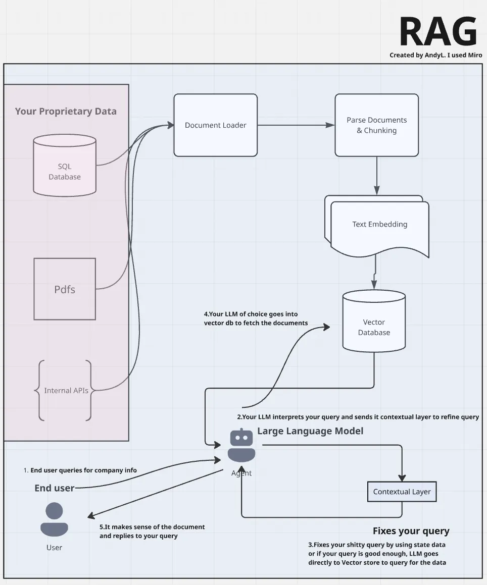
RAG or Retrieval augmented generation essentially unlocks the ability to feed your own proprietary or company data into the model’s thinking process. It retrieves relevant chunks of that data in real-time and augments the model’s response with it.
When you combine RAG with an LLM, you’re no longer limited to internet knowledge. You can build a chatbot that understands your product catalog, a virtual assistant that reads your internal documentation, or even a mini data analyst that answers questions based on reports and metrics your team actually uses. Basically, anything you can dream up that relies on your private data, RAG makes possible.
In this tutorial, we are going to build a simple RAG application using Langchain, a textbook will act as our data source
Step 1: Load your Data Source And Convert It Into a Document Object
In the Langchain ecosystem, there are plenty of document loaders to choose from. We need a pdf loader as our data source is a pdf.
Click to see other loaders available
"""
Loading the pdf and then converting it into a document object.
Each element represents a page hence there are 613 pages
if you check the length of the object.
"""

from langchain_community.document_loaders import PyPDFLoader

txtbook_path = "./statistics_txtbook.pdf"
loader = PyPDFLoader(txtbook_path)

docs = loader.load()

print(f"Our original textbook has {len(docs)} pages")
Step 2: Parse and Chunk the Document Object
We know that the textbook has a preface, table of contents, and a glossary/index section at the end. To save on costs, we should remove redundant information. After removing these pages, you should have 591 pages.
"""
Skipping preface,table of contents, and index.
Each document is a single page with varying length of text,
therefore we should exclude pages (1-11 inclusive both ends) and (603-613 inclusive both ends).
"""

cleaned_text_book = []
exclude_pages = set(range(0,12)) | set(range(603,614))
for doc in docs:
    page_num = doc.metadata.get("page",-1)
    if page_num in exclude_pages:
        continue
    cleaned_text_book.append(doc)


print(f"we are removing table of contents and index, we have {len(cleaned_text_book)} pages left")
Pages with less than a 100 words could potentially be worthless. To remove those pages we can use the .split() method. After removing these pages you should end up with 586 pages.
#remove pages with less than 100 words
useless_pages = []
filtered_docs = []
for doc in cleaned_text_book:
    page_num = doc.metadata.get("page",-1)
    if len(doc.page_content.split()) < 100:
        useless_pages.append((page_num,doc))
    else:
        filtered_docs.append(doc)

print(f"removing pages with less than 100 words, we have {len(filtered_docs)} pages")
Now that we parsed our data source to our liking, we need to determine if we should chunk the pages into smaller pieces. Smaller pieces improve query accuracy, wheras larger pieces help preserve context and meaning.
As of this moment, there isn’t a defined guideline and we are all still doing trial and error. I am going to go for a high context approach because statistical textbooks are generally technical and concepts can such as maximum likelihood and inference can span a dozen of pages. If you are following along, i.e using the same text-embedding model, you should have 1052 pages after chunking the document.
"""
Here, I'm checking the max length and average length of the set of documents,
the maximum length exceeds the token limitation so that's another
reason to chunk. (Note that text embedding models have token limitations)
"""
lengths = [len(doc.page_content) for doc in filtered_docs]
print(f"Average length: {sum(lengths)/len(lengths):.2f} characters")
print(f"Max length: {max(lengths)} characters")

"""
The chunk size and overlap is arbitrary, you're going to have to
do some trial and error to find the optimal performance.
We don't really have a guide line to benchmark this metric yet.
"""

from langchain_text_splitters import RecursiveCharacterTextSplitter

text_chunker = RecursiveCharacterTextSplitter(
    chunk_size = 2000,
    chunk_overlap = 500,
    separators=["\n\n", "\n", ".", "!", "?", ",", " ", ""]
)

docs_chunked = text_chunker.split_documents(filtered_docs)

print(f"we now have {len(docs_chunked)} pages because we reduced characters per page")
Step 3: Choose a Text-embedding Model and Insert Documents into Vector Database
In this step we are essentially transforming our text into vectors. We transform our text into vector’s because your queries are converted to vectors when you use an LLM. It’s a lot like regression, where we have a set of predictor values and a response variable. Whatever text-embedding model you choose, you’re going to have to stick with for the retrieval process. The third generation models are coming out soon but as of right now I am going to use text-embedding-ada-002 as it’s the cheapest option.
"""
I'm supplying the text embedding model to the embedding client.
Note: our text is not converted to vectors yet.
"""

from langchain_openai import OpenAIEmbeddings

text_embedding_model = "text-embedding-ada-002"

#make sure you have your key in your environment before you run this as it calls your key implicitly
embedding_function = OpenAIEmbeddings(
    model=text_embedding_model,
)
Now, before we convert our text into vectors and insert everything into the vector database in one pass, I’m going to break down the insertion proceess to smaller batches as there is an upper limit of 300k worth of tokens in a single upload.
# OpenAi has a 300k token limit, meaning that you can only upload 300k worth of token of
# documents at once, so to bypass that I am going to make multiple uploads in smaller sizes

batch_size = 100
initial_batch = docs_chunked[:batch_size]


from langchain_chroma import Chroma
#choose and create a vector database, I chose Chroma just cuz its the most used.
"""
document : gives the initial structure to the db
embedding: converts text into vectors
persist_directory: where we want to place the path of the vector database, also give it a name
(Note: it creates a new vector db if you misname this lol)
collection_name: essentially a table name for the document(s) cuz you can have different subjects,
not sure why you would want to but its there.
"""
vectorstore = Chroma.from_documents(
    documents=initial_batch,
    embedding=embedding_function,
    persist_directory="statisticsKnowledge.db",
    collection_name = "stats"
)

def batching_chunks(docs,size):
    for i in range(0,len(docs),size):
        yield docs[i:i+size]

#make sure to skip first batch because we already inserted it when defining the vector store.
for i,chunk_batch in enumerate(batching_chunks(docs_chunked[batch_size:], batch_size)):
    print(f"Adding batch {i + 2} of {len(docs_chunked) // batch_size + 1}")
    vectorstore.add_documents(chunk_batch)
Step 4: Make a query to your vector store
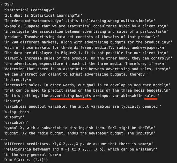
Now, to verify that our vector database is working correctly, we perform a similarity search to check if the LLM can retrieve documents relevant to our queries. To do this effectively, it’s best to query something very specific. For example, in this textbook, I know there’s a passage that explains potential predictor values for advertising. Although this detail might be redundant within the entire textbook, the goal is to ensure we can retrieve the exact document containing that information.
# Perform a similarity search for a specific query, returning the top 3 matches
# quick_sanity_check contains the top 3 documents that are most related to our query, order matters.
quick_sanity_check = vectorstore.similarity_search(
    query="When working with advertising data, what are potential predictor and response variables?",
    k=3
)

import pprint

# Ideally, the first retrieved document should be the most relevant and contain the answer
pprint.pprint(quick_sanity_check[0].page_content)
This is the output of the similarity search, we can tell that we did a good job because the first document contains our query’s answer.